


Charts in PivotXL provide a powerful way to make quick, data-driven decisions based on accounting reports. With dynamic chart visualizations, you can efficiently track your business’s financial progress and identify trends at a glance. PivotXL offers various chart types, making it easier to present and share key insights. The visual overview helps quickly identify potential issues, ensuring smarter business decisions with minimal effort.
Line Chart
Ideal for tracking changes over time, line charts provide a clear view of trends such as sales growth, expense patterns, or revenue fluctuations.
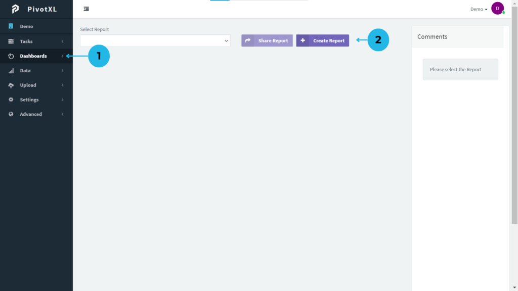
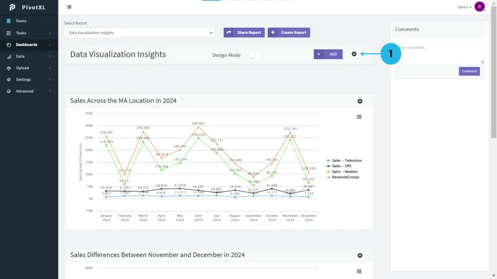
1.Access the PivotXL application and navigate to the Dashboards option from the left-hand menu to quickly create report charts for financial performance.
2.Click the Create Report button to generate a report, using various chart types to analyze financial data.
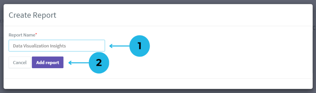
1.A pop-up will appear for creating the report. Enter a name based on your reporting needs.
2.Click the Add Report button to create a new report layout.
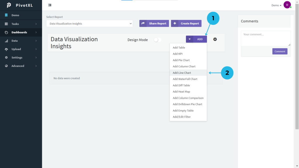
1.After creating the report, the ADD button becomes visible. Click it to explore all options for building your report.
2.Start by selecting the Add Line Chart option to create a line chart for your analysis.
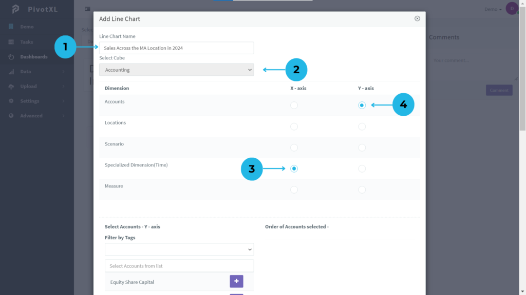
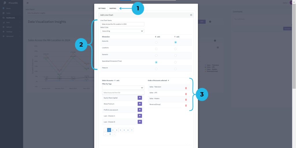
1.A new pop-up will appear for configuring the line chart. First, name the chart appropriately.
2.Choose the cube that aligns with your report requirements.
3.Assign Time as the X-Axis for chronological analysis.
4.Set Accounts Dimension as the Y-Axis for plotting financial data.
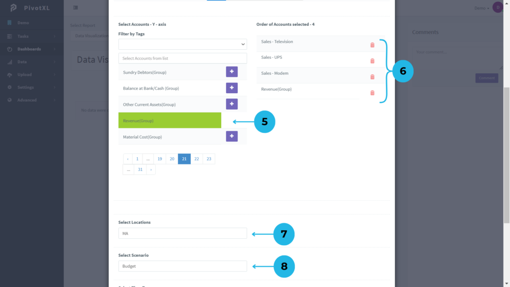
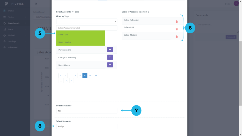
5.Select the accounts list for the Y-Axis. Click the plus icon to add them, turning green to indicate selection.
6.Review the selected accounts list, displayed in order, with the ability to modify as needed.
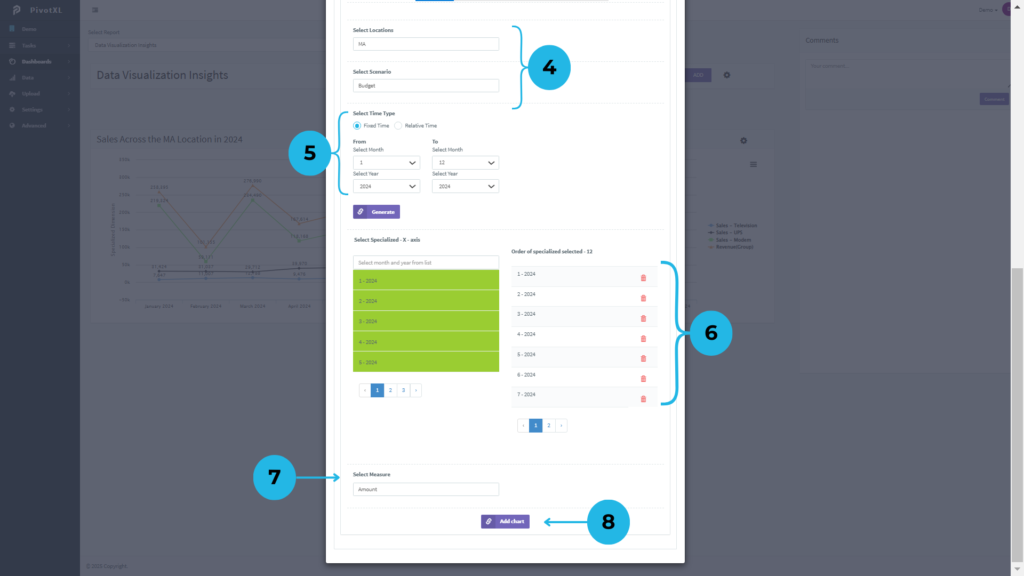
7.Choose MA as the Location Dimension for geographic filtering.
8.Set Budget as the Scenario Dimension to focus on planned financial performance.
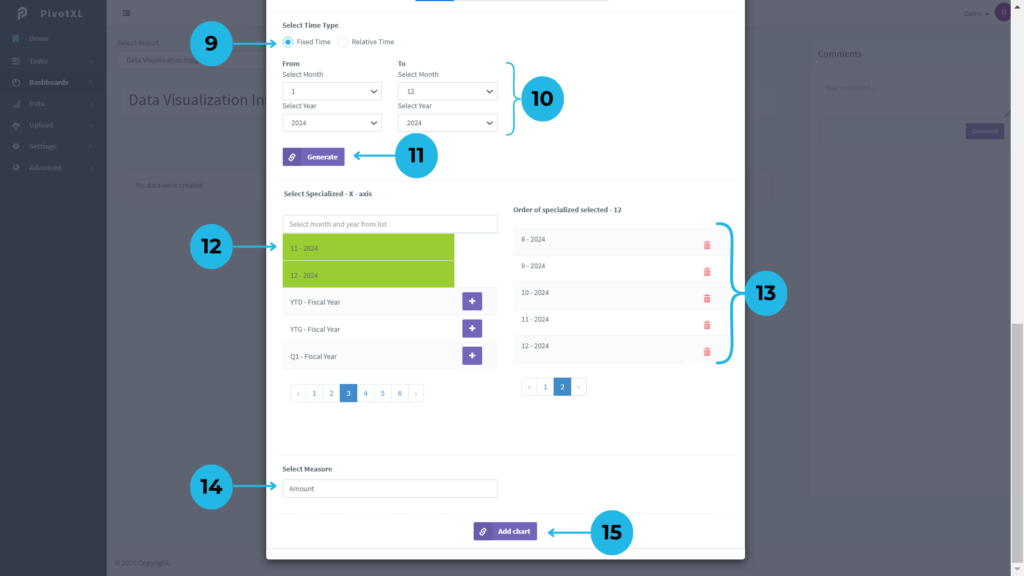
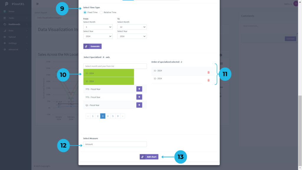
9.Choose Fixed Time as the Time Type for configuring the Line Chart.
10.Select the Month and Year, ranging from 1 to 12 months in 2024, for detailed time-based analysis.
11.Click the Generate button to create a list of months based on your selection.
12.Select the specialized X-Axis Months list. Click the plus icon to add them, with the color turning green to confirm selection.
13.The selected months will be displayed in the order of selection, along with a count of the months added.
14.Assign the Measure Dimension to Amount for accurate data representation.
15.Click the Add Chart button to create and display the Line Chart.
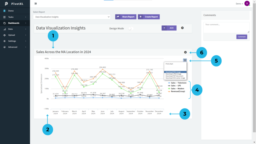
1.This is the Line Chart based on your prepared configurations, offering clear data visualization.
2.The chart is aligned with steps ranging from minimum to maximum values, including negative values if applicable.
3.Displays aligned data points for months 1 to 12 in 2024, enabling detailed time-based analysis.
4.Selected accounts are visually represented with distinct colors. You can click on an account name to make its line invisible on the chart for focused analysis.
5.Click the Options icon to download the Line Chart in various formats, such as PNG, JPEG, PDF, or SVG.
6.Click the Settings icon to seamlessly modify and update the chart’s configuration as required. This feature also displays all mappings, allowing you to edit and refine them with ease for precise customization.
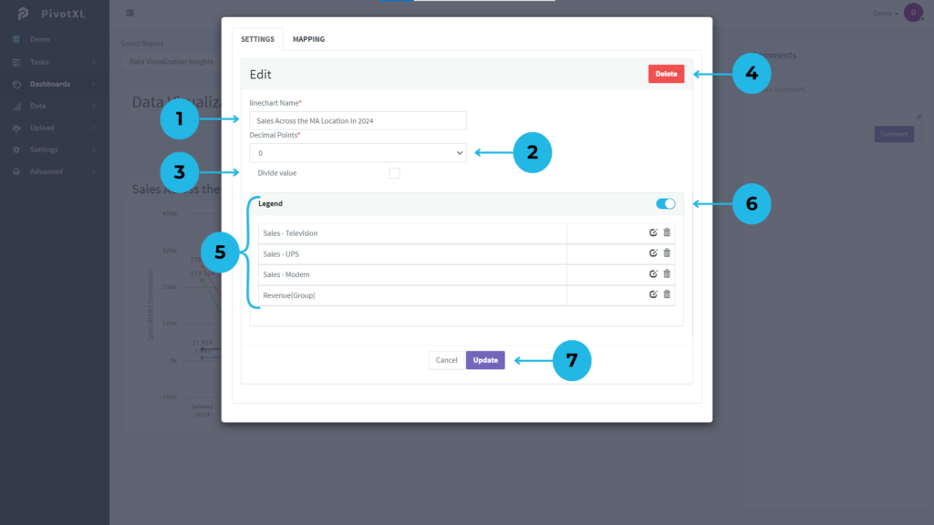
1.A new pop-up will open for configuring the Line Chart settings. Begin by making any required edits.
2.You can modify values to display decimals for greater precision in the chart.
3.Click the checkbox if you want to divide the values displayed in the chart for better readability.
4.Use the Delete button to permanently remove the Line Chart if it is no longer needed.
5.The Legend represents the list of accounts included in the Line Chart. You can modify account names or remove them by clicking the Edit or Delete icons.
6.Toggle the Enable/Disable option to control whether all accounts in the list are visible or hidden in the Line Chart.
7.Click the Update button to apply any modifications made to the Line Chart settings, ensuring an updated and accurate visualization.
1.Click on the MAPPINGS tab to view the structured setup of chart mappings.
2.Displays the chart name along with the selected X-axis and Y-axis configurations.
3.Lists the order of accounts applied on the Y-axis for clarity.
4.Highlights the selected Location and Scenario members within the dimensions.
5.Shows the chosen Time Type, including the specific Month and Year.
6.Displays the list of months selected under the Time Type settings.
7.Reflects the selected Measure Dimension member applied in the chart.
8.After modifying mapping details, click the Add Chart button to update with the new configurations.
Easily reorder and refine mappings to optimize chart presentation—details on this will be explained in the next chart section.
Column Chart
Best suited for comparing different categories, column charts display financial data side by side, making it easy to analyze performance across departments or periods.
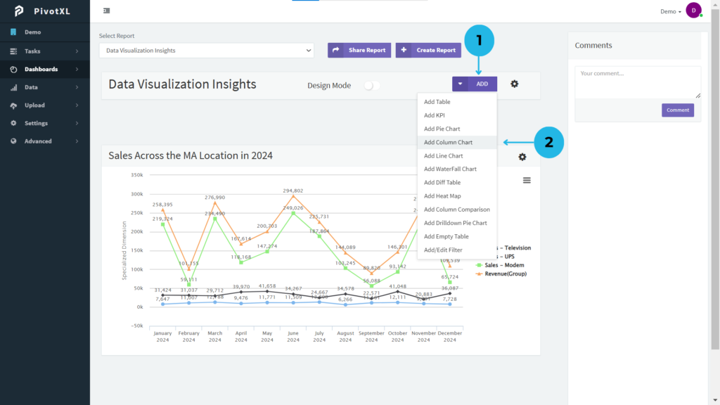
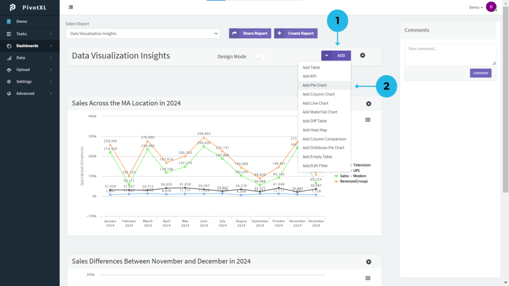
1.In the Dashboards report, click the ADD button to explore all the options for building and customizing your report.
2.Start by selecting the Add Column Chart option to create a Column chart for your analysis.
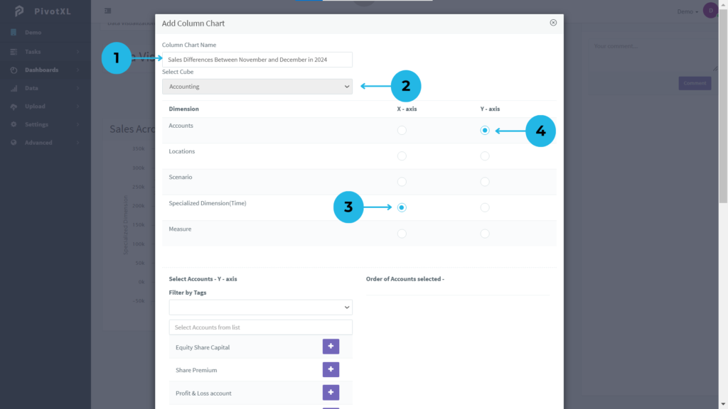
1.A new pop-up will appear for creating the Column Chart. Begin by entering a name for the chart.
2.Select the cube that matches your reporting needs.
3.Assign the X-axis to Specialized (Time) for time-based analysis.
4.Assign the Y-axis to the Accounts dimension.
5.Choose the desired accounts for the Y-axis, then click the plus icon. Once added, the selection will turn green, indicating successful inclusion in the Y-axis Accounts list.
6.Review and modify the selected Y-axis accounts list as needed.
7.Set the Location dimension to MA.
8.Choose the Scenario dimension as Budget.
9.Assign the time type to Fixed Time, select the year 2024, and specify months from 1 to 12. Click the Generate button to generate the months.
10.From the generated list, select the needed months, click the plus icon, and see the color change to green upon selection.
11.View the selected months in the order of selection, along with their count.
12.Assign the Measure dimension to Amount.
13.Click the Add Chart button to create the Column Chart for your report.
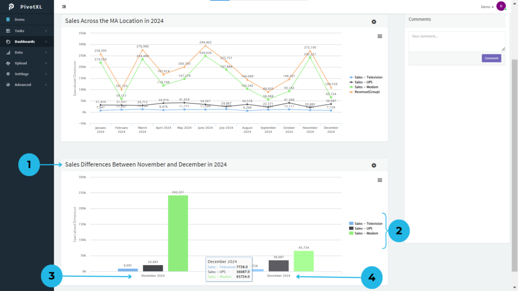
1.This Column Chart is built from your configured settings, providing clear and intuitive data visualization. It effectively compares the sales budgets for two months in a year.
2.Selected accounts are represented with distinct color bars. For focused analysis, click on an account name to hide its column from the chart.
3.The chart illustrates the November 2024 sales budget, with columns that represent values visually. Each column displays the exact value at its top for easy interpretation.
4.Similarly, the chart displays the December 2024 sales budget, with columns clearly showing corresponding values, prominently displayed above each column for precision.
5.Click the Options icon to download the Column Chart in various formats, such as PNG, JPEG, PDF, or SVG.
6.Click the Settings icon to seamlessly modify and update the chart’s configuration as required. This feature also displays all mappings, allowing you to edit and refine them with ease for precise customization.
Pie Chart
Perfect for showcasing proportions and distributions, pie charts help visualize how various components contribute to the whole, such as expense categories or revenue streams.
1.In the Dashboards report, click the ADD button to explore all the options for building and customizing your report.
2.Start by selecting the Pie Chart option to create a Pie chart for your analysis.
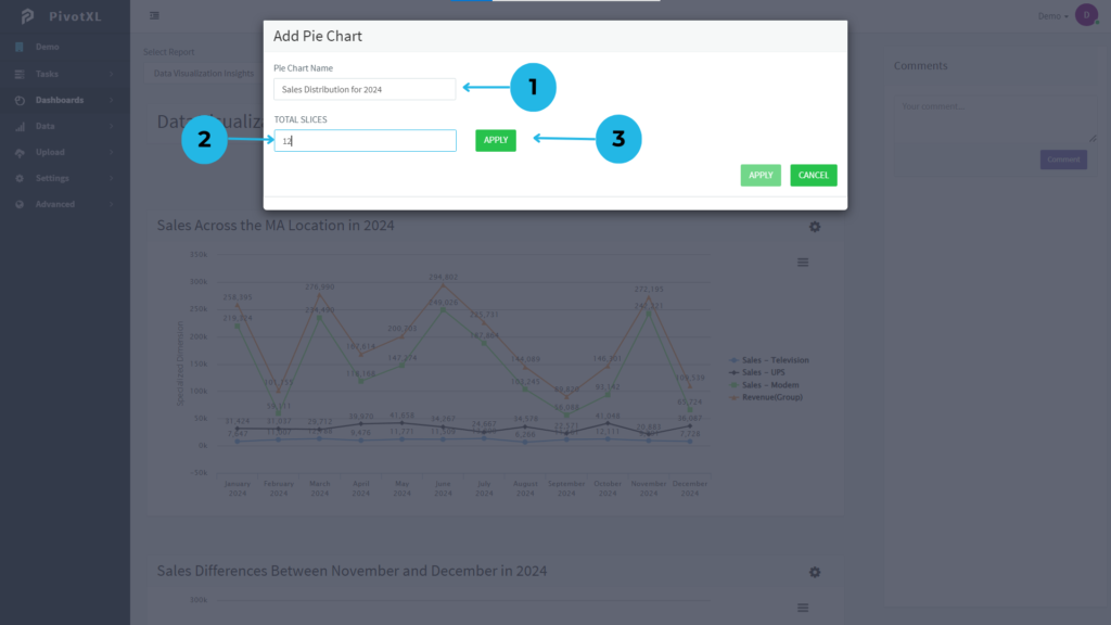
1.A new pop-up opens to begin creating your Pie Chart. Start by naming your chart to align with your reporting needs.
2.Utilize the TOTAL SLICES option to split the chart into segments. Simply enter the desired number of slices (e.g., 12) for tailored and precise data visualization.
3.Click the APPLY button to instantly generate the slices for your Pie Chart, making it ready for insightful analysis.
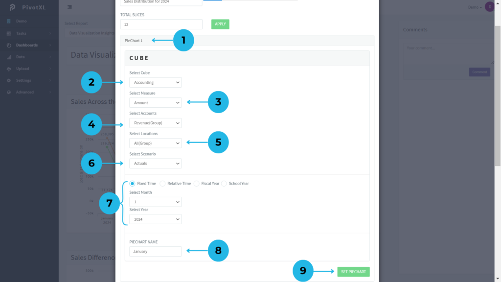
1.The slice names are automatically generated in the Pie Chart with a count (e.g., PieChart 1). Click on PieChart 1 to access its setup options.
2.Choose the Cube required for your Pie Chart’s data report.
3.Set the Measure Dimension to Amount for accurate value representation.
4.Assign the Accounts Tag Dimension to Revenue Group for categorization.
5.Select All Group for the Location Dimension, providing a holistic view.
6.Set the Scenario Dimension to Actuals for real-time data analysis.
7.Choose Fixed Time and select the Month and Year (e.g., January 2024, represented as 1 2024).
8.Give the slice a clear name for reference in the chart (e.g., January).
9.After ensuring all settings are correct, click the SETPIECHART button to save PieChart 1. Once saved, the button will become disabled, preventing further modifications.
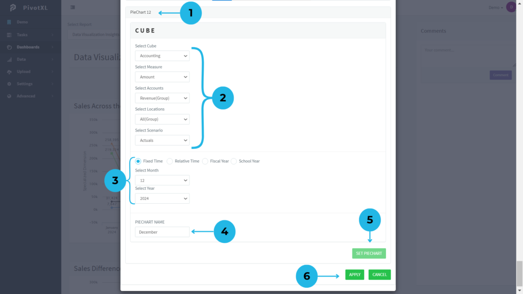
1.The 11 slices are already preconfigured with their respective cubes and dimensions in the PieChart slices. This step involves setting up the final slice of the Pie Chart, which will be appropriately named (e.g., December).
2.Use the same Cube and Dimension settings as previously configured for other slices.
3.Update the Month and Year for this slice to December 2024.
4.Assign a meaningful name to the Pie Chart slice in PIECHARTNAME (e.g., December) for easy identification.
5.After confirming all settings, click the SETPIECHART button to save PieChart 12. Once saved, this button will become disabled, ensuring no further modifications can be made.
6.Once all slices are configured and finalized, click the APPLY button to create the complete Pie Chart Report. This step consolidates all the slices into a cohesive and visually impactful report.
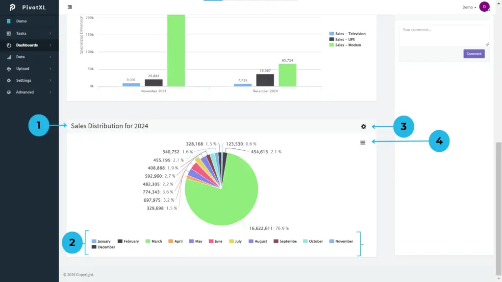
1.The Pie Chart is displayed as part of the report, offering clear insights into the data.
2.Each slice is uniquely labeled with a name and represented by distinct color variations in order. All slices showcase their values as a percentage of the Pie Chart’s total, enabling quick comprehension of proportions.
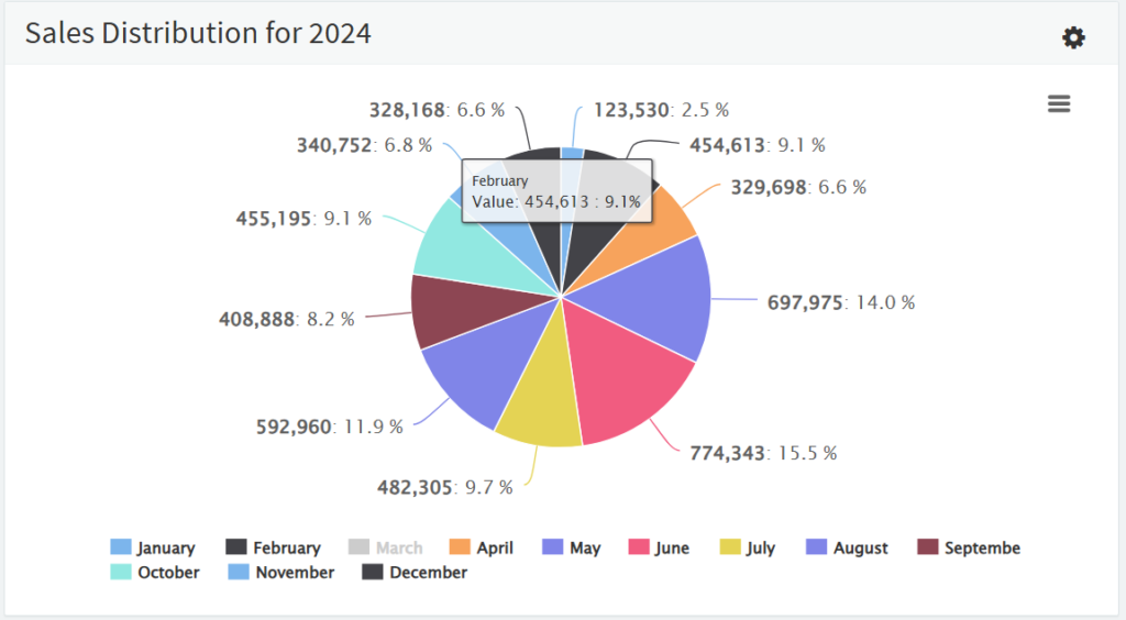
The March slice has been disabled, leaving the other 11 slices active in the chart.
3.Click the Settings icon to seamlessly modify and update the chart’s configuration as required. This feature also displays all mappings, allowing you to edit and refine them with ease for precise customization.
4.Click the Options icon to access various download formats, including PNG, JPEG, PDF, and SVG, for convenient sharing or offline use.
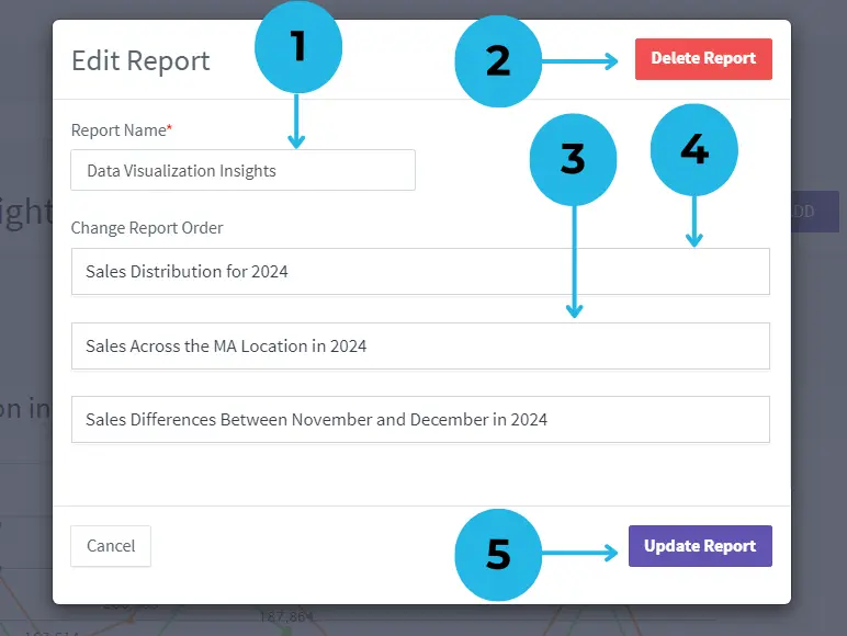
1.Use the Report Settings Icon to edit the report name, rearrange chart orders, or delete charts seamlessly.
- Update the report name anytime to keep it relevant and organized.
- Remove unnecessary reports by clicking the Delete button for a clutter-free workspace.
- Drag and drop charts to adjust their order in the report effortlessly
- Move the Pie Chart to the top for better visibility or reposition the Line Chart to suit your report’s flow.
- Ensure all updates are finalized by clicking the Update Report button, locking in your modifications.
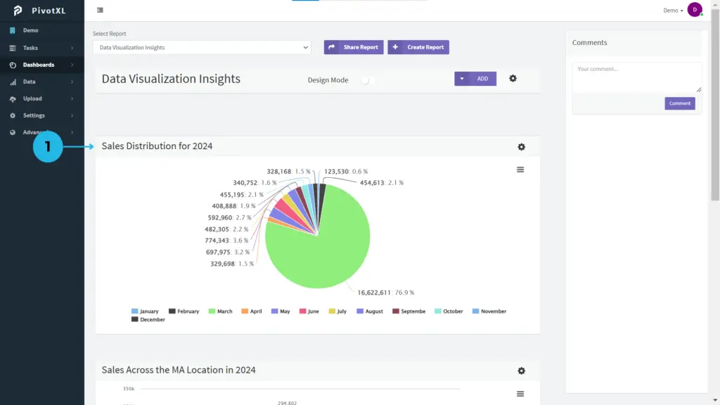
1.The modified report now reflects the new arrangement, with the Pie Chart prominently displayed at the top for instant visibility and impact.
Present and Share Insights
PivotXL makes it easy to share your insights with stakeholders by providing visually appealing and interactive charts. Whether you’re preparing a financial presentation or analyzing operational trends, these charts ensure your data is both accessible and impactful.
Unlock the power of visual storytelling with PivotXL charts, and transform your data into actionable insights effortlessly.