


Are you working with a lot of data in Excel and need to make specific rows stand out? If so, you’re not alone—many professionals, from analysts to administrators, often face the challenge of making large datasets more readable and easier to interpret. Whether you’re organizing monthly sales figures, tracking employee attendance, managing inventory records, or preparing a comprehensive report, knowing how to highlight multiple rows in Excel can significantly improve your workflow and save valuable time. In fact, this simple yet powerful feature enhances not just the visual clarity of your spreadsheet but also the way you interact with your data on a daily basis.
Additionally, highlighting rows makes it much easier to compare values, spot discrepancies, and draw meaningful conclusions at a glance. Furthermore, it allows you to quickly identify important trends, patterns, and outliers that may otherwise go unnoticed in a sea of numbers. With that in mind, mastering techniques such as manual highlighting, conditional formatting, and dynamic formatting rules can give you much greater control over how your data is displayed.
With just a few simple steps, you can dramatically enhance the visual structure of your worksheet, streamline navigation, and ultimately boost your overall productivity. All in all, learning how to highlight multiple rows in Excel is a practical and versatile skill—one that can make a significant difference in both your efficiency and the quality of your data analysis.
In this easy-to-follow tutorial from PivotXL, we’ll guide you through simple steps to highlight multiple rows in Excel — no experience required! Let’s get started.
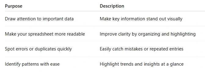
Why Highlight Rows in Excel?
Highlighting rows helps:
Method 1: Manually Highlighting Multiple Rows
For small datasets, manual highlighting is often the easiest option.
Step-by-Step Instructions for Highlight Multiple Rows:
- Open your Excel file.
- Click and drag your mouse to select the rows you want to highlight.
Tip: Hold the Ctrl key while clicking to select non-adjacent rows. - With your rows selected, go to the Home tab.
- Click the Fill Color icon (paint bucket).
- Choose the color you want to use.
Method 2: Highlight Rows Using Conditional Formatting
This method is great for automatically highlighting rows based on certain conditions.
Step-by-Step Instructions for Highlight Multiple Rows:
- Select the entire dataset (including the rows and columns).
- Go to the Home tab.
- Click on Conditional Formatting > New Rule.
- In the dialog box, choose “Use a formula to determine which cells to format.”
- Enter a formula like:
=$C2>100This will highlight rows where the value in Column C is greater than 100. - Click Format, choose a highlight color, and click OK.
Result:
Now, any row where the value in Column C is more than 100 will be highlighted automatically.
Method 3: Highlight Every Other Row (For Readability)
This is especially useful for large spreadsheets. Excel can do this automatically using a built-in table style.
Step-by-Step Instructions for Highlight Multiple Rows:
- Select your data range.
- Press Ctrl + T to convert your data into a table.
- In the dialog box, make sure “My table has headers” is checked (if applicable), then click OK.
- Excel will now format your data and automatically highlight every other row.
Practical Example: Highlight Sales Over $5,000
To illustrate, let’s say you have a list of monthly sales, and you’re looking to highlight all rows where the sales figures exceeded $5,000.
- Select your data.
- Go to Conditional Formatting > New Rule.
- Use this formula: bashCopyEdit
=$B2>5000 - Choose a bold color like green, then click OK.
Quick Tips for Beginners
- Use Ctrl + Click to select multiple non-adjacent rows.
- Undo formatting by pressing Ctrl + Z or using the “Clear Rules” option under Conditional Formatting.
- Use themes to keep colors consistent and professional.
Final Thoughts
Knowing how to highlight multiple rows in Excel can significantly boost your productivity and make your data easier to understand. Whether you’re doing it manually or using conditional formatting, Excel provides a wide range of powerful tools to help you customize and manage your spreadsheet more effectively. Not only does this improve the visual appeal, but it also makes working with large data sets far more intuitive. In addition to enhancing aesthetics, these techniques allow you to visually organize vast amounts of information, making patterns, trends, and outliers much easier to identify.
As a result, you can draw insights more quickly and avoid missing critical details. In the same vein, when you become comfortable with row highlighting, you can greatly streamline your data analysis process and enhance the overall clarity of your reports. What’s more, this skill can save you time and reduce errors when dealing with complex datasets. Ultimately, it’s a straightforward yet impactful way to gain better control over how your data is presented, interpreted, and used for decision-making. In summary, mastering row highlighting is a small step that can lead to big improvements in your workflow and data accuracy.
To dive deeper, learn more about Highlight Multiple Rows on Excel and discover additional tips to make your data analysis even more effective.