


A clustered column chart in Excel is a highly useful tool that makes it easy to compare multiple sets of data side by side. Whether you are analyzing sales figures, survey responses, or business trends, this chart type helps you clearly identify patterns, trends, and differences within your data. By organizing information visually, it allows for quick and effective analysis, making decision-making much easier. In this step-by-step guide, we will walk you through the entire process of creating a clustered column chart in Excel in a simple, easy-to-understand, and practical way.
What is a Clustered Column Chart in Excel?
Example Use Case:
A clustered column chart in Excel can be used in various ways to simplify data analysis. For example, it is helpful for comparing monthly sales of multiple products, allowing businesses to track performance trends over time. Additionally, it is useful for analyzing student test scores across different subjects, making it easier to identify strengths and areas for improvement. Furthermore, this chart type is great for visualizing annual revenue by department, helping organizations assess financial performance and allocate resources more effectively.
Steps to Create a Clustered Column Chart in Excel
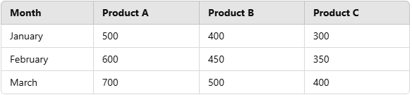
Enter Your Data
Follow these easy and straightforward steps to quickly create a Clustered Column Chart in Excel. By following this process, you can efficiently visualize and compare data, making your analysis clearer and more insightful. Let’s get started!
Insert a Clustered Column Chart
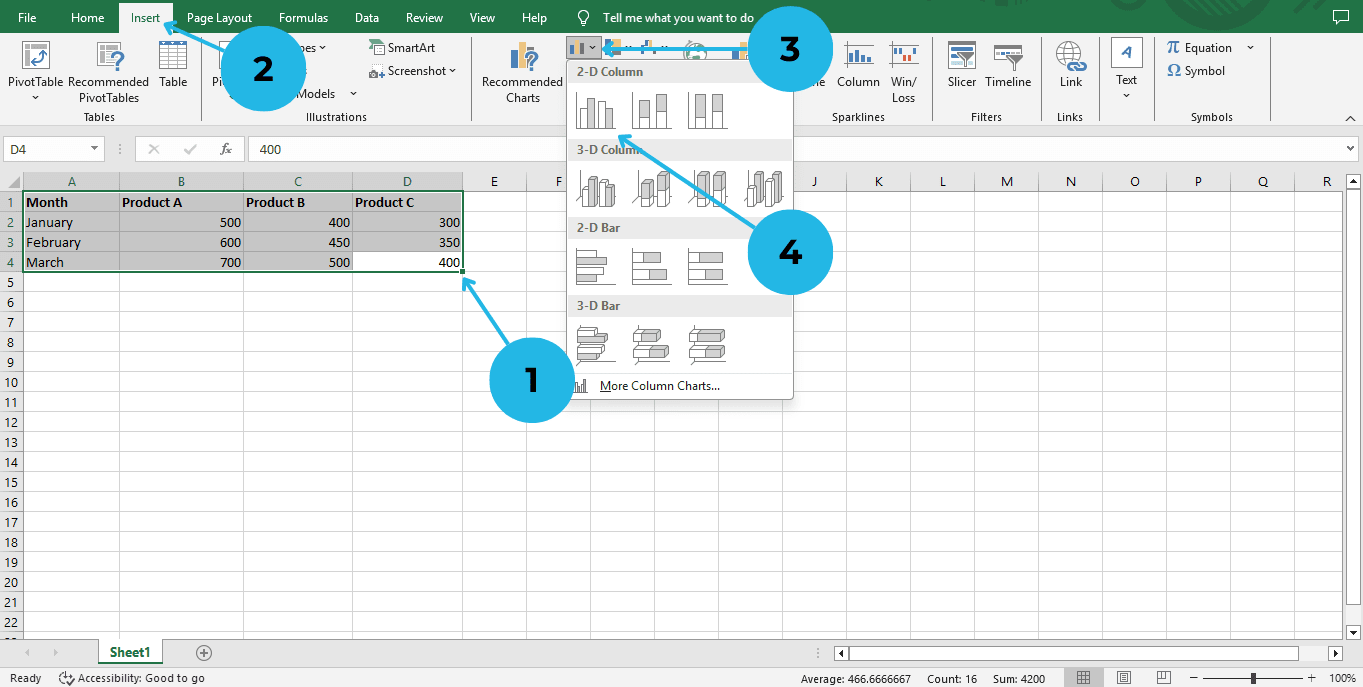
- Click and drag to select your dataset
- Go to the Insert tab on the Excel ribbon.
- Click on Insert Column or Bar Chart.
- Select Clustered Column Chart from the dropdown.
At this point, Excel will generate a basic clustered column chart.
Customize the Chart
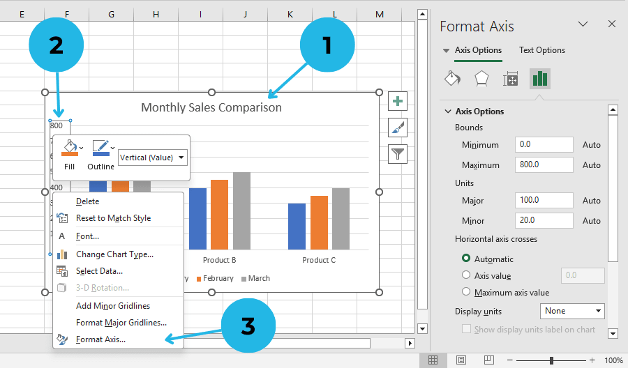
- Add a Chart Title: Click on the chart title and type a descriptive title (e.g., “Monthly Sales Comparison”).
- Adjust the Axis Labels: Right click on the horizontal axis labels.
- Click on Format Axis and customize the labels.
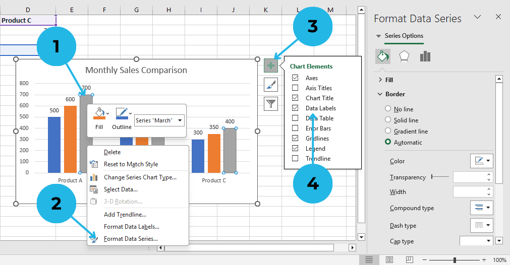
- Change Colors and Styles: Right click on the bar.
- Click on Format Data Series and choose different colors or styles to enhance readability.
- Add Data Labels: Click on Chart Elements(+ icon).
- Select Data Labels to display values directly on bars.
Best Practices for Clustered Column Charts
To begin with, keep your Clustered Column Chart simple by limiting the number of data series to avoid clutter. Next, use contrasting colors to make each data series visually distinct, ensuring better readability. By following these key guidelines, you can create a clear and effective chart that enhances data visualization. Additionally, label your chart clearly by making axis labels and legends easy to understand. Finally, sort your data logically so that categories are arranged in a meaningful order, making analysis more efficient and insightful.
Conclusion
Creating a clustered column chart in Excel is not only simple but also a highly effective way to visually present comparative data. By carefully following these step-by-step instructions, you can easily transform raw numbers into meaningful insights that are easier to understand and analyze. Furthermore, using this chart type allows you to highlight key trends and patterns, making your data-driven decisions more informed. So, why not try it out with your own dataset? With just a few clicks, you can enhance your reports and presentations by creating clear, visually appealing, and professional-looking charts that leave a lasting impact!
Learn more about the Stacked Bar Chart in Excel by using our PivotXL website. This powerful chart type helps you compare data segments within a whole, making analysis easier and more insightful. So, explore its features today and enhance your data visualization skills with PivotXL!