


Have you ever seen the error #N/A in Excel and wondered how to handle it? If so, don’t worry — you’re not alone! Dealing with errors in Excel can seem confusing at first, but with the right tools, it becomes much easier. Fortunately, there’s a simple function that can help: ISNA in Excel. Next, we’ll dive into step-by-step instructions with clear examples to show you how it works in real situations. Along the way, you’ll also find practical tips to help you avoid common mistakes and make your spreadsheets cleaner and more professional. Moreover, we’ll show you how to combine ISNA with other functions like IF, so you can create smarter formulas that handle errors automatically. By the end of this guide, you’ll feel confident using ISNA to troubleshoot #N/A errors and improve your overall Excel skills. So, let’s get started and transform your spreadsheets today!
What is ISNA in Excel?
ISNA is a special function in Excel that checks if a cell has the #N/A error.
If the cell has the #N/A error, ISNA returns TRUE; if not, it returns FALSE.
Learn more about how to use ISNA Function to handle errors and keep your spreadsheets clean and professional.
Tip: “#N/A” means Not Available — it usually happens when a formula like VLOOKUP can’t find a value.
Why Use ISNA in Excel?
- To catch and manage errors in your data.
- To create cleaner reports without ugly error messages.
- To combine with other functions like IF, for smarter formulas.
Syntax of ISNA
Here’s what the ISNA formula looks like:
=ISNA(value)
- value: This is the cell or formula you want to check.
Step-by-Step: How to Use ISNA in Excel
Let’s go through a real example to make it super easy!
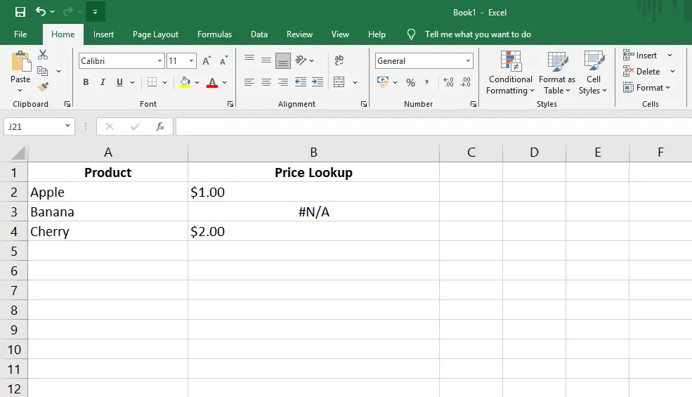
Example 1: Basic ISNA Check
Imagine you have a list where you tried to look up product prices, but some products are missing.
Step 1:
Click into a new empty cell where you want your ISNA result.
Step 2:
Type the formula:
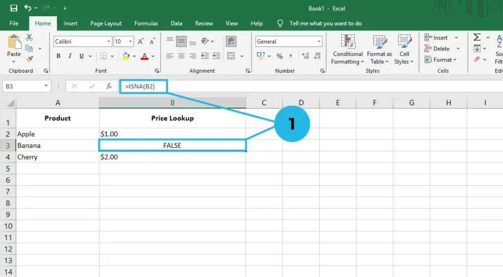
=ISNA(B2)
(Here, B2 is the cell you are checking.)
Step 3:
Press Enter.
- If B2 is #N/A, it will show TRUE.
- If B2 has a value, it will show FALSE.
Example 2: Using ISNA with IF
Now, let’s make it even smarter!
You can use ISNA with IF to show a custom message instead of an error.
Formula:
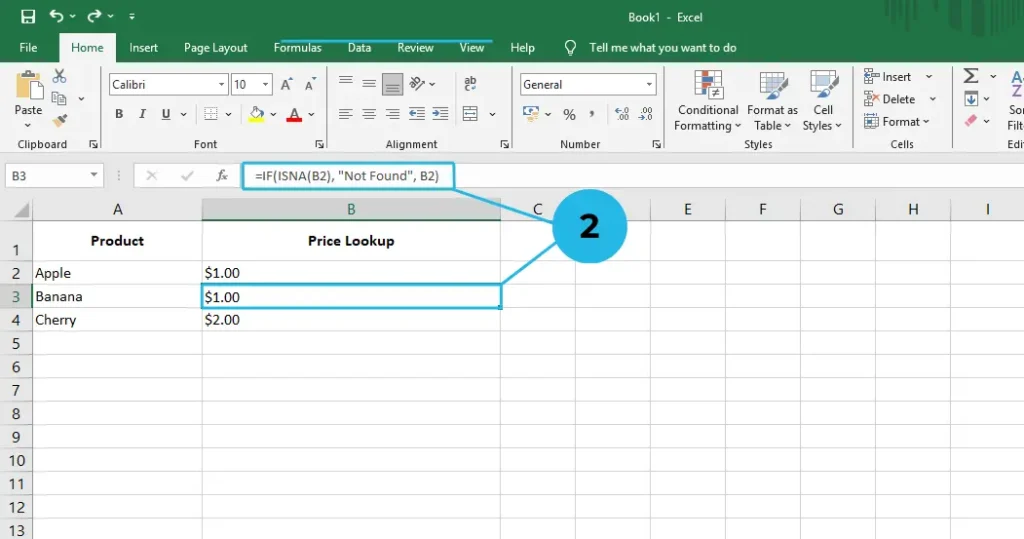
=IF(ISNA(B2), "Not Found", B2)
This says:
- If B2 has an error, show “Not Found“.
- Otherwise, show the actual value.
Where ISNA is Most Useful
- VLOOKUP or XLOOKUP errors: When data is missing.
- Data Cleaning: Checking for missing or broken entries.
- Dashboards: Hiding errors for cleaner visuals.
Bonus Tip: Use IFNA Instead!
Excel also has a function called IFNA, which is even simpler!
=IFNA(B2, "Not Found")
- It automatically checks for #N/A without needing ISNA and IF separately.
Conclusion: Master Errors with ISNA in Excel!
Learning how to use ISNA in Excel is an important skill that helps you handle errors smoothly and efficiently. As a result, your spreadsheets will not only look cleaner but will also be much easier to read and understand. In fact, by catching and managing #N/A errors early, you can prevent small mistakes from turning into larger problems later on. Moreover, using ISNA ensures that your reports, dashboards, and data analysis are both accurate and professional-looking. Whether you are working on a simple project or a complex data report, mastering ISNA can save you valuable time and effort. Additionally, combining ISNA with functions like IF allows you to create smart formulas that automatically replace errors with meaningful messages. Therefore, learning ISNA not only improves your technical Excel skills but also boosts your overall productivity.
In short, by adding ISNA to your Excel toolbox, you can quickly transform messy, error-filled spreadsheets into clean, reliable, and polished documents with ease. Not only does it help you catch and fix errors, but it also improves the overall quality and professionalism of your work, making your data easier to read, understand, and share.
Practice these examples, and soon, those pesky #N/A errors won’t bother you at all!
Liked this tutorial? Explore more Excel tips and tricks at PivoXL!