


When working with Excel, you might often encounter errors like #DIV/0!, #VALUE!, or #N/A. These errors can make your spreadsheet look messy and confusing. Fortunately, Excel provides a simple solution: the IFERROR function. In this guide, we will explain what the IFERROR function is, how it works, and how you can use it effectively in your spreadsheets. So, let’s dive in!
What is the IFERROR Excel Function?
The IFERROR function in Excel is used to catch and handle errors in formulas. Instead of displaying an error message, you can replace it with a custom value, such as a blank cell, text, or an alternative calculation.
Learn more about IFERROR Excel Function.
Syntax of IFERROR Function
=IFERROR(value, value_if_error)
- value: The formula or expression to evaluate.
- value_if_error: The value to return if the formula results in an error.
Why Use the IFERROR Excel Function?
- Improves readability: Prevents distracting error messages from appearing, making your spreadsheet easier to understand.
- Enhances data presentation: Displays meaningful values instead of errors, ensuring a cleaner look.
- Helps with calculations: Ensures that calculations continue smoothly even when errors occur, which is particularly useful in complex spreadsheets.
How to Use IFERROR in Excel (Step-by-Step)
Let’s go through a simple example to see how the IFERROR function works in Excel.
Example 1: Handling Division by Zero Error
Imagine you have a dataset where you need to divide numbers, but some denominators are zero. This can cause errors, but IFERROR can help.
Enter Data:
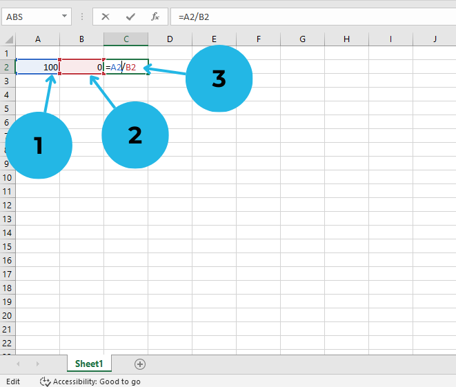
- In A2, enter
100(numerator). - In B2, enter
0(denominator). - In C2, enter the formula
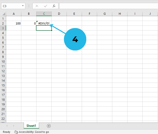
=A2/B2. - This results in a
#DIV/0!error.
Apply IFERROR:
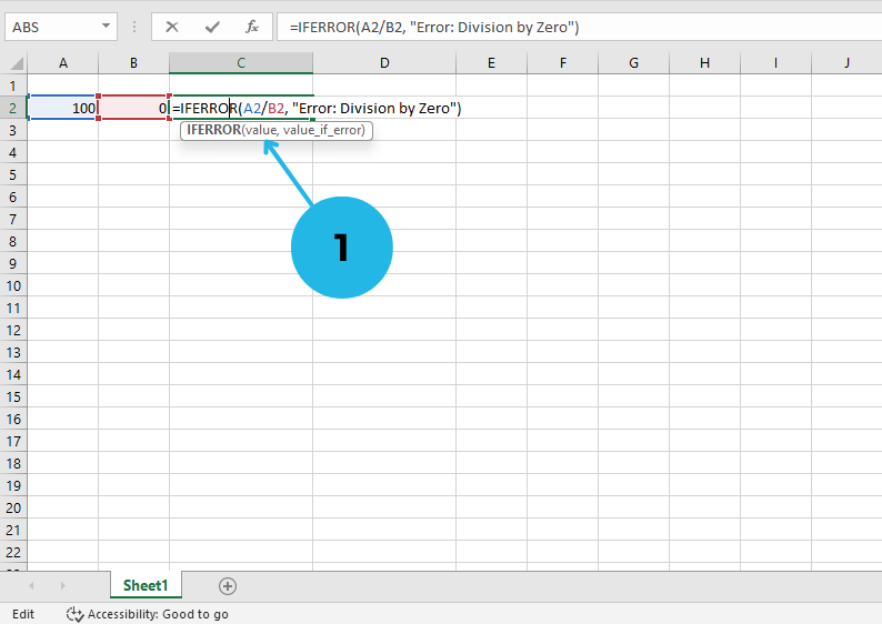
- Modify the formula in C2:
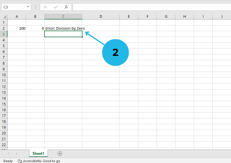
=IFERROR(A2/B2, "Error: Division by Zero") - Instead of
#DIV/0!, you will now see:Error: Division by Zero. As a result, your spreadsheet looks much cleaner!
Example 2: Replacing Errors with a Default Value
Sometimes, you might want to replace errors with a default value like 0. This is especially helpful when performing calculations that rely on error-prone formulas.
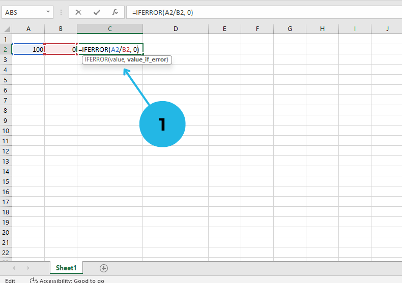
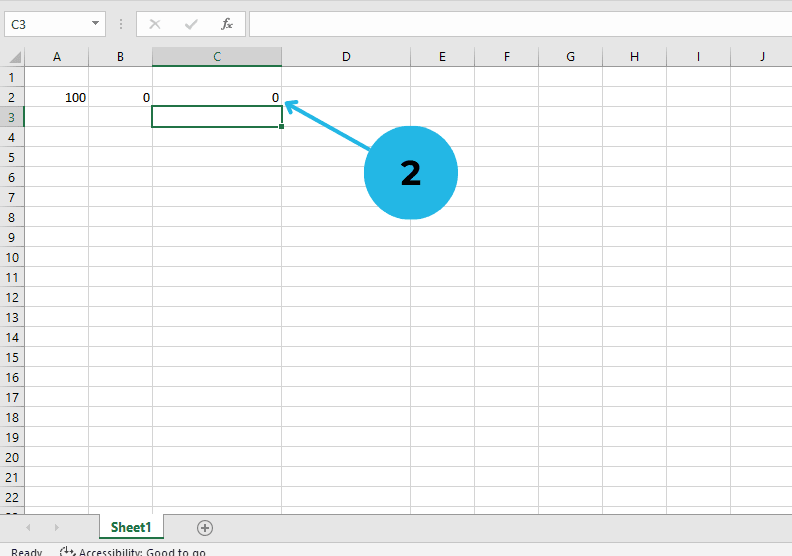
- Use the formula:
=IFERROR(A2/B2, 0). If there’s no error, the correct value is displayed. - If an error occurs,
0appears instead of an error message. This way, your calculations remain intact.
Example 3: Using IFERROR with VLOOKUP
When using VLOOKUP, you might encounter #N/A errors if a value isn’t found. Luckily, you can use IFERROR to return a custom message instead.
- Assume your data is in columns A and B.
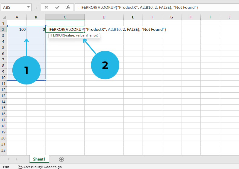
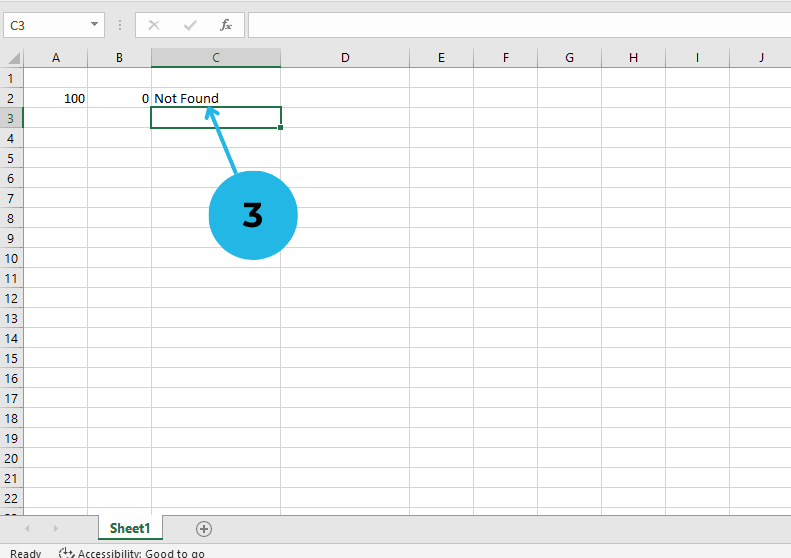
- Use the formula:
=IFERROR(VLOOKUP("ProductX", A2:B10, 2, FALSE), "Not Found") - If “ProductX” exists, it returns the corresponding value. Otherwise, it shows “Not Found” instead of
#N/A. This makes it much easier to understand missing data.
Best Practices for Using IFERROR
- Use it sparingly: While IFERROR is useful, overusing it can hide real issues in your data. Instead, investigate why errors occur in the first place.
- Combine with other functions: You can use IFERROR with
VLOOKUP,AVERAGE,SUM, and many more functions to make your formulas more reliable. - Customize error messages: Instead of a generic message, provide helpful text that explains the issue. This way, users can quickly understand what went wrong.
Conclusion
The IFERROR Excel function is a powerful tool for managing errors and improving spreadsheet usability. By using IFERROR, you can keep your data clean and readable while preventing unwanted error messages from disrupting your workflow. So, why not try using it in your spreadsheets today? With a little practice, you’ll be able to handle Excel errors effortlessly!
For more Excel tips and tutorials, stay tuned to PivotXL!