


What are Roll-ups?
Roll-ups are a way to assign dimension members to specific tags in a cube’s dimension. This process helps create higher-level summaries of data by aggregating detailed data points into broader categories.
Assigning Dimension Members to Roll-Ups
Assigning dimension members to roll-ups involves linking specific dimension members to a group within a designated tag, based on the roll-up category within that dimension and cube.
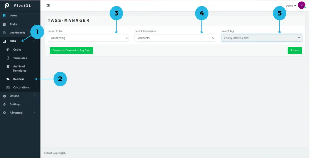
1. Data
Click on Data in the left-side menu.
2. Roll-ups
Click on Roll-Ups under the Data menu. You will see the page for adding dimensions to tags.
3. Select Cube
Click the dropdown and select the cube you want to work with.
4. Select Dimension
Click the dropdown and select the dimension you want to assign to a tag.
5. Select Tag
Click the dropdown and select the dimension tag. If you haven’t created any dimension tags yet, the dropdown will be empty.
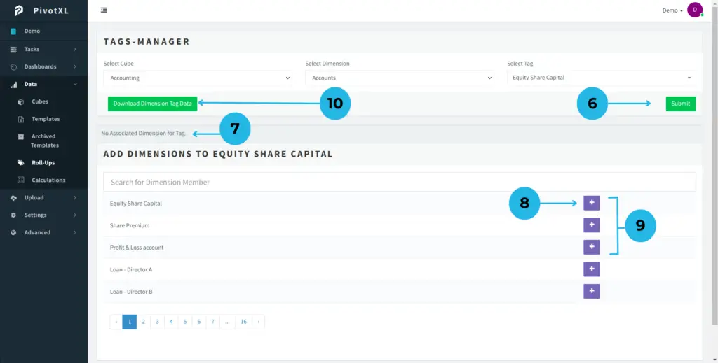
6. Submit
Once you have selected the cube, dimension, and dimension tag, click the Submit button.
7. No Assigned Dimension Members
If no dimension members are assigned to this dimension tag yet, a message will indicate “No Associated Dimension for Tag”.
8. Add Dimension Button
You will see a list of all dimension members for the selected dimension. Click the plus icon next to the dimension member you want to add to the dimension tag.
9. Add Dimensions To Tag
Add the first three dimensions to the selected dimension tag.
10. Download Dimension Tag Data
Click the download button. This will download a CSV file containing details of which tags are assigned to each dimension member.
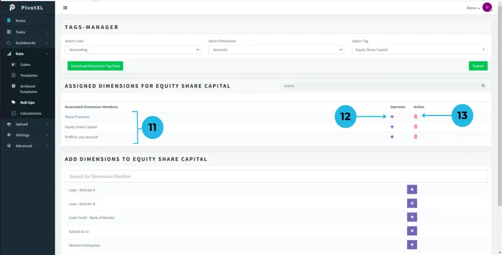
11. Assigned Dimensions for Dimension Tag
This section shows the list of dimension members that have been assigned to the selected dimension tag.
12. Operator
The operator allows you to change the aggregation method for the tag. By default, the plus (+) icon indicates a positive number. If you want to change the values from positive to negative for a specific dimension member, click the plus (+) icon to switch it to a minus (-) icon. This operator change affects only the selected tag and not other tags.
13. Action
If you want to remove a member from the tag, click the delete icon.
Assigning Dimension Members to Roll-Ups in PivotXL (Video Tutorial)
Mapping Roll-Ups in Excel
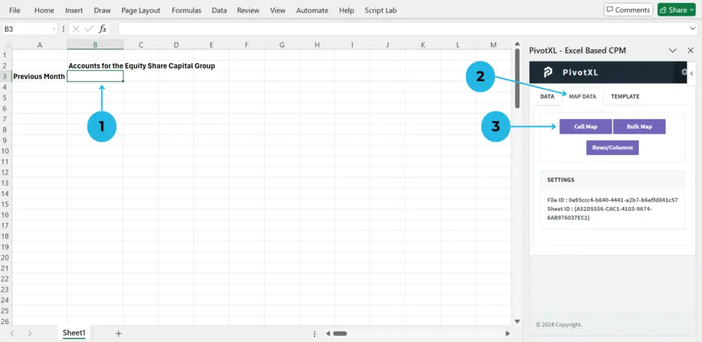
1.Click on the cell you want to map in your Excel sheet. Open the PivotXL Add-in and log in.
2.In the PivotXL toolbar, click the Map Data button.
3.Click the Cell Map button to display the mapping options.
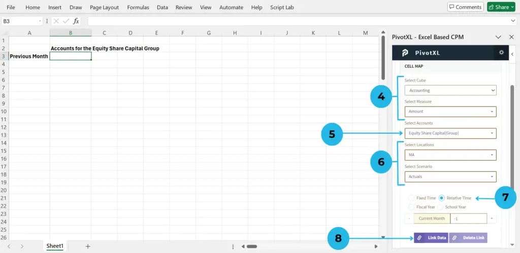
4.Choose the relevant cube and measure for your mapping.
5.Select the Accounts Dimension. Choose the Dimension Tag in which you want to group dimension members for this mapping.
- Tip: Dimension Tag names include “(Group)”.
- Example: Select “Equity Share Capital (Group)” if you have grouped ‘Accounts’ dimension members under this tag.
6.Choose the dimensions for Location and Scenario to include in your mapping.
7.Select the dimension for Relative Time to map data for the previous month.
8.Click the Link Data button to connect your mapping to the database.
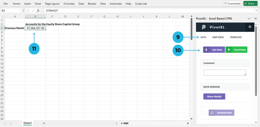
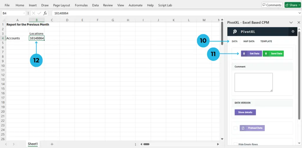
9.Click on the Data button to retrieve data for the mapped cell.
10.Click the Get Data button to fetch the data.
11.The values for the mapped dimension combinations will be displayed. If the combinations do not exist, it will show as empty. The tag works with the members included in the Grouping Dimension Members and calculates the values shown in the cell, including all values within the grouped Dimension Members.
Mapping Roll-Ups Across Multiple Dimensions
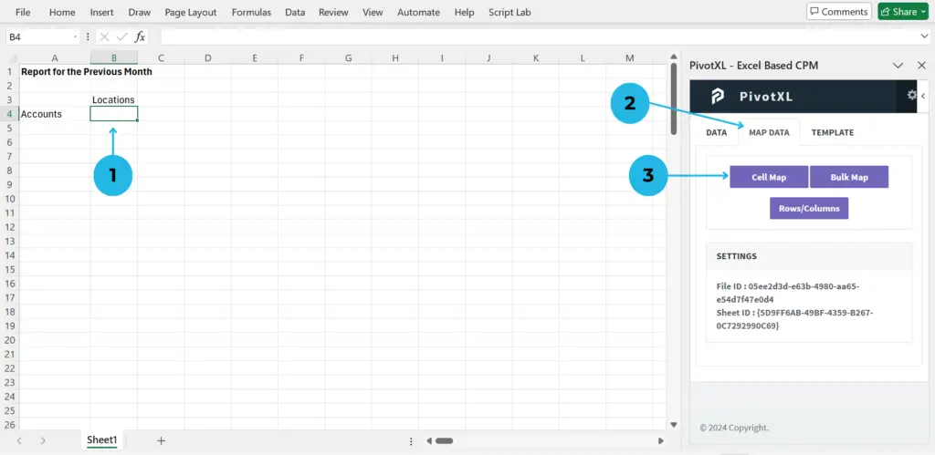
1.Begin by clicking on the cell in your Excel sheet where you want to map your data.
2.In the PivotXL toolbar, locate and click the Map Data button.
3.Click the Cell Map button to display the mapping options available for the selected cell.
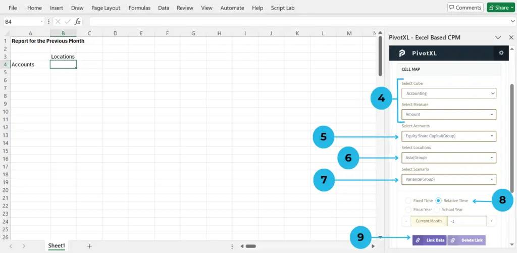
4.In the mapping options, choose the relevant cube and measure for your data mapping.
5.Select the Accounts Dimension. Choose the appropriate Dimension Tag where you want to group dimension members.
- Tip: Dimension Tag names include “(Group)”.
- For example, select “Equity Share Capital (Group)” if you have grouped ‘Accounts’ dimension members under this tag.
6.Select the Locations Dimension. Choose the appropriate Dimension Tag that represents the groupings you need.
7.Select the Scenario Dimension. Choose the appropriate Dimension Tag that represents the groupings you need.
8.Select the dimension for Relative Time to map data for the previous month.
9.Click the Link Data button to save the mappings.
10.Click the Data button to retrieve data for the mapped cell.
11.Click the Get Data button to fetch the data.
12.The values for the mapped dimension combinations will be displayed in the cell. If the combinations are not available, the cell will show as empty.
How to Effectively Drill Down into Cells for Detailed Insights
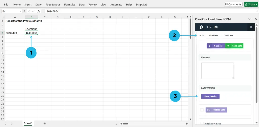
1.Start by clicking on the cell in your Excel sheet where you want to drill down the value by grouping.
2.Click on the Data button in the toolbar.
3.Click the Show Details button to open a new pop-up window that displays the drill-down cell value.
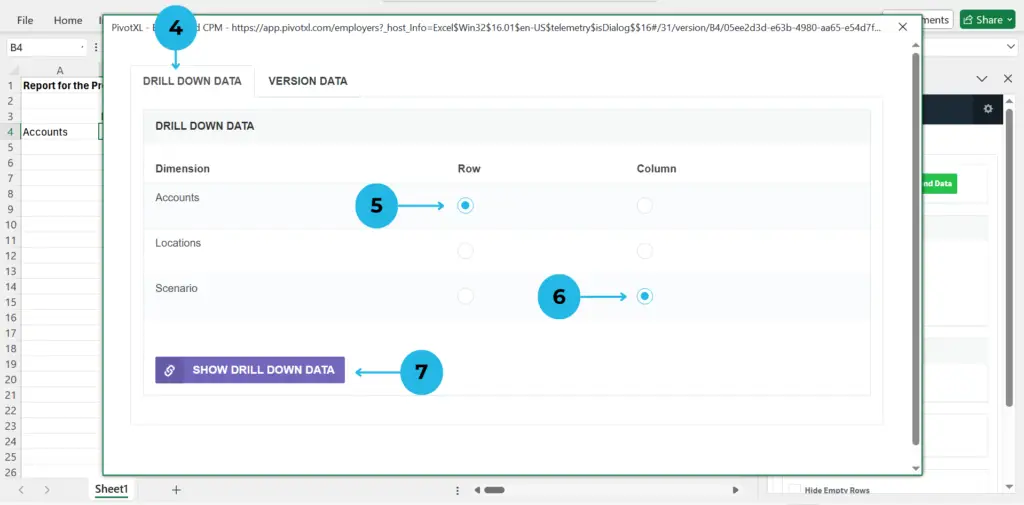
4.In the pop-up window, navigate to the Drill Down Data tab.
5.Choose Accounts for the row selection.
6.Select Scenario for the column selection.
7.Click the Show Drill Down Data button, showing a new tab below. This drill-down shows the breakdown of accounts and scenarios in the selected cell value.
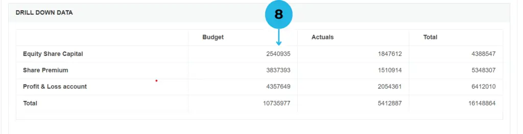
8.In the Drill Down Data tab, you’ll see accounts as rows and scenarios as columns, complete with totals. Click on the value for ‘Equity Share Capital’ and budget to further break it down by the Locations group dimension tag, which opens a new tab.
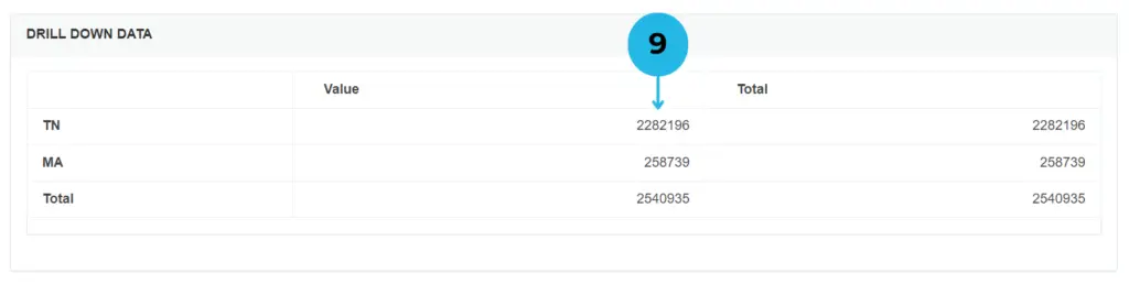
9.Review the detailed data from the locations dimension for the grouped values. Click on the TN value to open a new tab for version details.
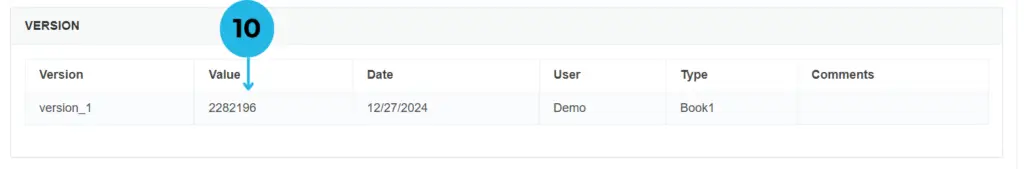
10.If the drill-down process has concluded, you will see a detailed view of the value combination, including version, value, date, user, type, and comments.